I Spent 8 Iterations Prompt-Engineering an LLM to Read 20-Pixel Icons. A 2005 Algorithm Did It Better.
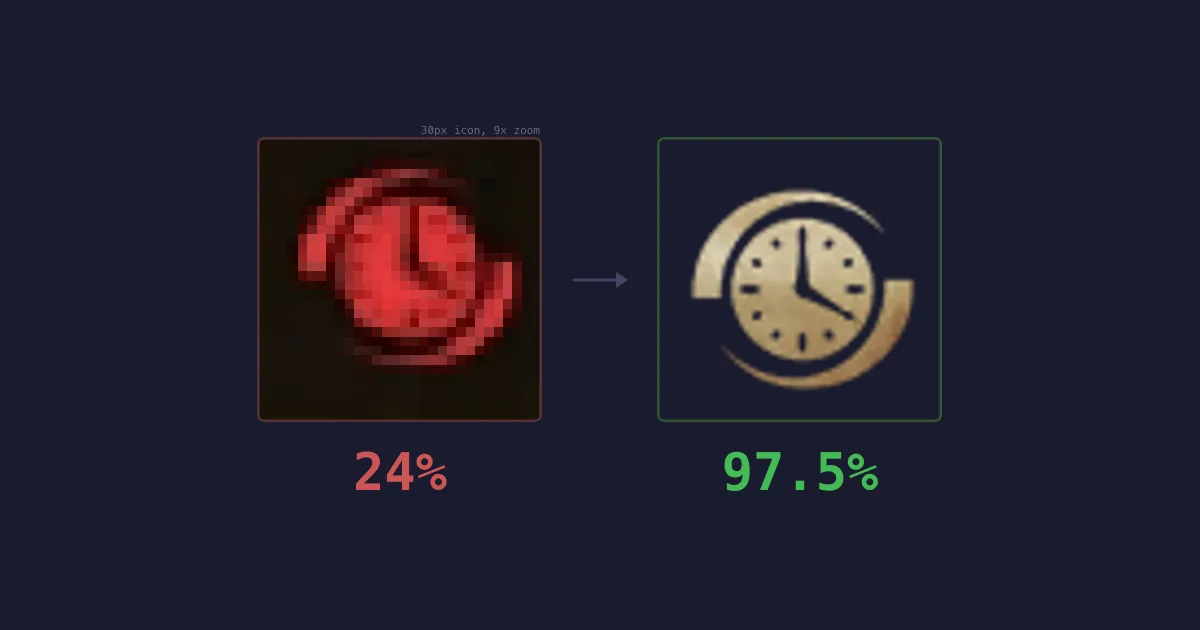
The most expensive AI model on earth scored 17% identifying tiny game icons. The model one tier below it scored 24%. A gradient histogram algorithm from 2005, written in 170 lines of TypeScript, scored 97.5%. It also ran 100x faster and cost me nothing.
This is the story of how I learned that lesson - and why I think it matters beyond gaming.
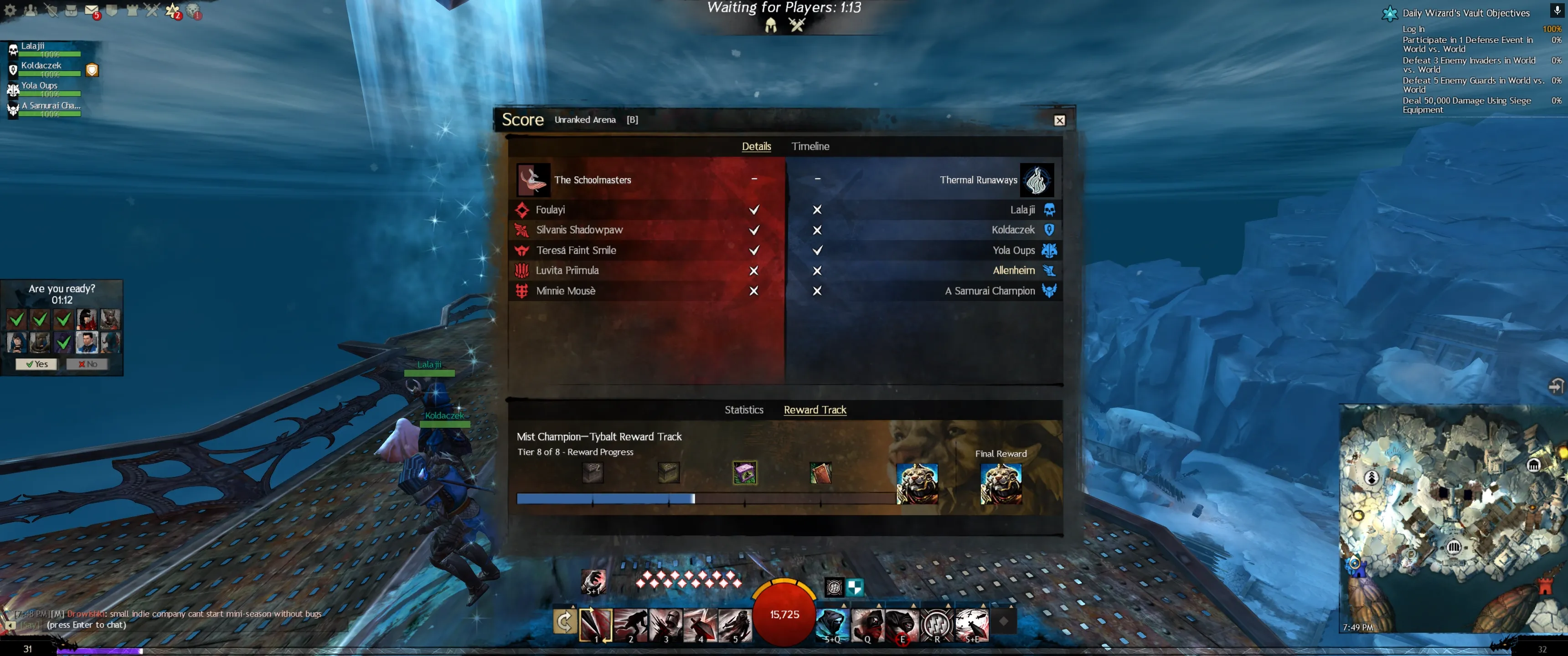
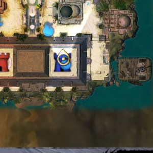
I play Guild Wars 2, a competitive online game. Before each PvP match, you get about 60 seconds to study a scoreboard showing 10 players - their names and character classes, displayed as small icons. It changes the way you and your team should play.
I built a desktop app that reads a screenshot of this scoreboard and streams real-time tactical advice from an LLM. The hard part wasn’t the advice. It was reading the screenshot.
Each character class is represented by a ~20-pixel icon - an abstract silhouette sitting on a coloured team background. There are 45 possible classes, many with similar shapes. Red team icons sit on a red gradient that absorbs most colour information, leaving only the faintest outline.
The whole scan has to complete in seconds to make any sense. You’re racing a countdown timer.
Act 1: Teaching an LLM to See
My first prototype sent the screenshot to Claude’s vision API. One API call, structured output - done. No specific image processing, no feature engineering - you just describe what you want and let the model figure everything else out.
Here’s what 8 iterations of prompt engineering looked like:
| Iteration | What I Changed | Name Accuracy | Icon Accuracy |
|---|---|---|---|
| 1 | ”Analyse this scoreboard” (naive) | 16% | 20% |
| 2 | Described the layout structure | 34% | 5% |
| 3 | Upgraded from Haiku to Sonnet 4.0 | 50% | 15% |
| 4 | Line-by-line layout + system prompt | 83% | 15% |
| 5 | Upgraded to Sonnet 4.6 | 99% | 30% |
| 6 | Added chain-of-thought reasoning | 99% | 33% |
| 7 | Sent a labelled reference chart of all 45 icons | 98% | 53% |
| 8 | Tried PNG, higher res, disambiguation rules, Opus | 99% | 17%-55% |
These are profession-level numbers (9 classes). Keep reading.
Names: solved. Sonnet 4.6 reads names at 99%. The jump from Haiku (16%) to Sonnet 4.6 (99%) was far larger than any prompt improvement within the same model.
Icons: stuck. After 8 rounds, accuracy plateaued. The error distribution was bimodal - specific icons were either correct 90%+ of the time or 0% of the time.
The single biggest improvement was sending a reference chart (all 45 icons in a labelled grid) as the second image:
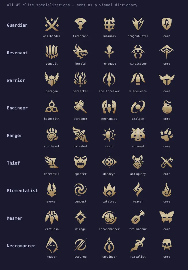
This nearly doubled accuracy from 30% to 53%. But then I discovered something worse.
I was measuring the wrong thing the whole time. My test harness graded against 9 base professions when the scoreboard actually shows 45 elite specialisations. I was checking “is it a dog?” instead of “what breed?” When I corrected the evaluation, 53% collapsed to 24% (29/120 across 3 runs).
Bigger models made it worse. Opus (the most capable model) scored 17%. It deliberated, second-guessed correct reads. It hallucinated a “spider-like icon” that doesn’t exist in the game and presented it as an answer. For a narrow pattern matching task like this, thinking harder was simply counterproductive.
Disambiguation rules backfired. Telling the model “don’t confuse thief with guardian” fixed that pair but destabilised everything else. Accuracy dropped from 53% to 42%. The model over-applied the rules elsewhere.
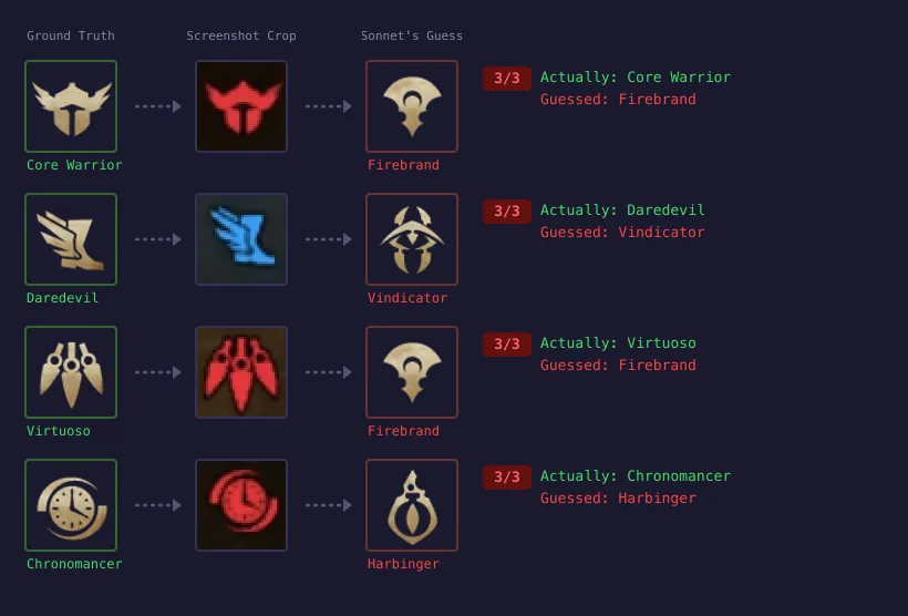 At 20 pixels, daggers and blades are the same shape. The LLM guessed wrong three out of three times.
The icons were truly physically ambiguous at 20 pixels and no amount of verbal reasoning could resolve that.
Act 2: Going Old-School
I switched to HOG (Histogram of Oriented Gradients) - a feature extraction algorithm from 2005. It computes gradient directions in small image cells and builds orientation histograms. The result captures shape while ignoring colour and lighting - just what I needed for matching noisy coloured crops against clean reference silhouettes.
We had 170 lines of TypeScript, no OpenCV, no TensorFlow, no cloud API, no training data, one reference image per class and a whole galaxy of multi-coloured game screenshots. Not that we needed all that for the win, but once you get locked into a serious project, the tendency is to push it as far as you can. (Full implementation on GitHub.)
97.5% - 39 out of 40 icons correct. 40 milliseconds for 10 icons. $0 per scan. Deterministic.
But here’s the part that surprised me most. The first version of this same algorithm only scored 65%. Same code, same references.
The problem was upstream. Icon crops were being extracted at slightly wrong positions - off by a few pixels. On a 35-pixel crop, that means the icon is partially cut off, surrounded by background noise. When I fixed the crop pipeline - template matching for an anchor point, calibrated pixel offsets per UI size - accuracy jumped from 65% to 97.5% without changing a single line of the classifier.
The classifier was fine from day one. It was sitting downstream of sloppy input extraction.
I’ve seen this pattern in every data engineering role I’ve held. Most accuracy problems aren’t model problems, they’re data pipeline problems.
The Comparison
| LLM Vision (Sonnet 4.6) | Local CV Pipeline | |
|---|---|---|
| Icon accuracy | 24% (29/120) | 97.5% (39/40) |
| Name accuracy | 99% | ~80% (correction UI) |
| Latency | 3-5s (API) | ~3.5s (all local) |
| Cost per scan | ~$0.02 | $0 |
| Deterministic | No (varies per run) | Yes |
| Debuggable | No (black box) | Yes (inspect features) |
The final system uses both. Local CV handles everything that needs to be fast, accurate, and deterministic. The LLM handles what it’s actually good at: reading names (99%) and generating strategic reasoning from structured input.
Total calibration data for the entire pipeline: ~50 files, under 1MB.
What I’d Tell You Over Coffee
If you’re building a system that needs to classify a known set of visual patterns from constrained inputs, try the boring approach first. Not because LLMs can’t do vision - they can, impressively - but because general-purpose reasoning is overhead when your problem is specific.
HOG was published in 2005. It runs in 40 milliseconds. It requires zero training data - just one reference image per class. It’s deterministic, so when it’s wrong, you can inspect the feature vectors and understand why. When accuracy drops on new inputs, you adjust a crop offset or add a reference image. You don’t retrain a model or pray that your next prompt cracks 60%.
The LLM approach cost me 8 iterations of prompt engineering and produced a system that was wrong three-quarters of the time. The classical approach cost me 170 lines of straightforward math and produced a system that’s right 97.5% of the time.
Sometimes the 2005 algorithm is the 2026 solution.
Appendix: How the Pipeline Actually Works
The narrative ends above. What follows is for the engineers who want to know how each piece works. The full source is on GitHub.
Anchor Detection (~1.7s)
The scoreboard is a draggable window. I find its close button (X) via NCC template matching - 4 templates for 4 UI sizes (21-28px). NCC is extremely peaky for small templates: correlation drops from 1.0 to ~0.55 at just 1-2 pixels offset. A coarse-to-fine search (scan every 4th pixel, refine) misses the peak entirely. Full pixel scan, narrowed to a search region, is the only correct approach. When multiple X buttons appear (Options panel, popups), team colour validation disambiguates: only the scoreboard has red and blue team columns at the predicted positions. 23/23 = 100%.
Map Detection (~15ms)
Crop the minimap (bottom-right corner, 300x300), downscale to 16x16 RGB, cosine similarity against stored thumbnails. The downscale is the denoising - player markers blur out, terrain colours survive. Each map has a unique palette. Each map has exactly one game mode, so map detection gives mode for free - eliminating a Y-coordinate heuristic that failed on 5/23 screenshots.

Drag to compare. The 16×16 pixel blob on the right achieves 100% map detection accuracy.
Layout (<1ms)
8 calibrated presets (4 UI sizes x 2 game modes), fixed pixel offsets from the anchor. Average position error: 2.27px across 230 crops.
OCR (~2.8s)
Tesseract.js with 4-worker pool. Each step in the preprocessing chain exists because its absence caused a specific bug:
// Scale 3x (crops too small for Tesseract)
.resize(crop.width * 3, crop.height * 3, { kernel: 'lanczos3' })
// White-on-dark -> black-on-white
.negate()
// Binarise
.threshold(128)
Then: trim black borders, re-pad 15px white, set DPI 150. The trim step was the non-obvious one - after negate + threshold, the scoreboard background becomes large black regions that Tesseract interprets as “nothing here.” Trimming black before padding with white took accuracy from ~50% to ~80%.
Bugs That Cost Hours
Sharp’s silent channel promotion. sharp.resize() on grayscale silently outputs 3-channel RGB. The metadata lies (channels: 1), but the buffer is 3x. HOG reads interleaved RGB as grayscale, garbage features, random classifications. Fix: .grayscale() after every .resize().
The Y coordinate lie. Game mode detected from anchor Y position. Failed on 5/23 screenshots because the scoreboard is draggable. Fix: detect the map instead - mode comes for free.
Weapon skill hallucination. The LLM advice layer confidently listed weapon skills the player didn’t have. Fix: fetch exact skill names from the game’s official API and inject as ground truth. Hallucinations: eliminated.